39 display the data labels on this chart above the data markers quizlet
quizlet.com › 295934888 › excel-flash-cardsExcel Flashcards | Quizlet A format that changes the appearance of a cell—for example, by adding cell shading or font color—based on a condition; if the condition is true, the cell is formatted based on that condition, and if the condition is false, the cell is not formatted. Exp19_Excel_Ch03_CapAssessment_Movies_Instructions.docx Add category and percentage data labels in the Inside End position. Turn off all other label indicators such as value and legend. Apply 14 pt font size and Black, Text 1 font color. 5 5 You want to focus on the comedy movies by exploding it and changing its fill color.
Exp19_Excel_Ch03_CapAssessment_Movies_Instructions | Chegg.com Remove value data labels and the legend. Apply 14 pt font size and Black, Text 1 font color You want to focus on the comedy movies by exploding it and changing its fill color Explode the Comedy slice, by 7% and apply Dark Red fill color 5 6 2 A best practice is to include Alt Text for accessibility compliance.

Display the data labels on this chart above the data markers quizlet
CIS Ch3 Excel Flashcards | Quizlet Apply the Monochromatic Palette 2 color scheme from the Monochromatic section.. Add data labels to the selected pie chart. Add a trendline to the chart. Switch the data series with the categories on this chart. 1. change the selected chart to cluster column chart. 2. change the selected chart to cluster column chart. Overview of PivotTables and PivotCharts - support.microsoft.com PivotCharts display data series, categories, data markers, and axes just as standard charts do. You can also change the chart type and other options such as the titles, the legend placement, the data labels, the chart location, and so on. Here's a PivotChart based on the PivotTable example above. For more information, see Create a PivotChart. How to make a histogram in Excel 2019, 2016, 2013 and 2010 - Ablebits.com So, let's get to it and plot a histogram for the Delivery data (column B): 1. Create a pivot table To create a pivot table, go to the Insert tab > Tables group, and click PivotTable. And then, move the Delivery field to the ROWS area, and the other field ( Order no. in this example) to the VALUES area, as shown in the below screenshot.
Display the data labels on this chart above the data markers quizlet. Solved PLEASE SHOW ALL | Chegg.com The chart needs a descriptive title that is easy to read. Type April 2021 Downloads by Genre as the chart title, apply bold, 18 pt font size, and Black, Text 1 font color. 5. 4. Percentage and category data labels will provide identification information for the pie chart. Add category and percentage data labels in the Inside End position. Types of Graphs - Top 10 Graphs for Your Data You Must Use Add data labels #8 Gauge Chart The gauge chart is perfect for graphing a single data point and showing where that result fits on a scale from "bad" to "good." Gauges are an advanced type of graph, as Excel doesn't have a standard template for making them. To build one you have to combine a pie and a doughnut. A Complete Guide to Line Charts | Tutorial by Chartio One way of doing this is through the addition of error bars at each point to show standard deviation or some other uncertainty measure. Another alternative is to add supporting lines above or below the line to show certain bounds on the data. These lines might be rendered as shading to show the most common data values, as in the example below. Excel sparklines: how to insert, change and use - Ablebits.com On the Insert tab, in the Sparklines group, choose the desired type: Line, Column or Win/Loss. In the Create Sparklines dialog window, put the cursor in the Data Range box and select the range of cells to be included in a sparkline chart. Click OK. Voilà - your very first mini chart appears in the selected cell.
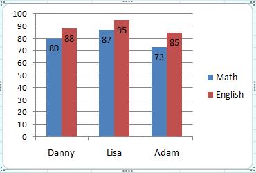
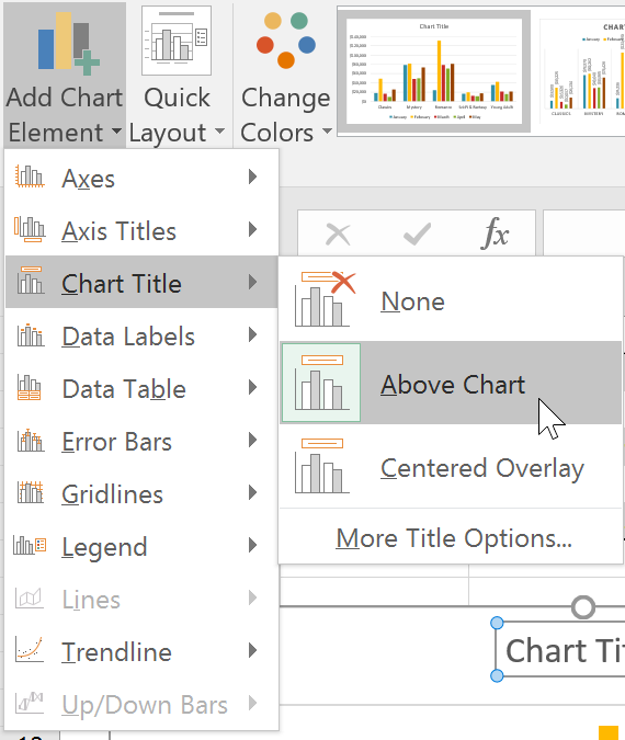
Show or hide a chart legend or data table Show or hide a data table. Select a chart and then select the plus sign to the top right. To show a data table, point to Data Table and select the arrow next to it, and then select a display option. To hide the data table, uncheck the Data Table option. The columns and pie slices in the charts above are - Course Hero The columns and pie slices in the charts above are ____. a. data markers c. major tick marks b. chart areas d. minor tick marks ANS: A PTS: 1 REF: EX 171 14. Referring to the figure above, the rectangular area to the right of the piechart (listing Cash, U.S. Stocks, Non-U.S. Stocks, and Bonds) is the ____. a. Solved 1 Open the Excel workbook | Chegg.com Computer Science questions and answers. 1 Open the Excel workbook Student_Excel_3F_Streets.xlsx downloaded with this project. 2 Change the Theme Colors to Blue Green. On the Housing Revenue sheet, in the range B4:F4, fill the year range with the values 2016 through 2020. 3 In cell Co, construct a formula to calculate the percent of increase in ... For Pre-test_week3 - 1 Click any of the data markers to... On the Chart Tools Design tab, in the Data group, click the Switch Row/Column button. 9 Display the data labels on this chart above the data markers. Click the Chart Elements button. Click the Data Labels arrow and select Above. 10 Display the data table, including the legend keys. Click the Chart Elements button and click the Data Table check box. 11 Add a new linear trendline to this chart. Use the default trendline type and formatting. Click the Chart Elements button that appears near the ...
quizlet.com › 392427351 › excel-flash-cardsexcel Flashcards | Quizlet Display the data labels on this chart above the data markers. You launched the Chart Elements menu. In the Mini Toolbar in the Data Labels menu, you clicked the Above menu item. Markers | Maps JavaScript API | Google Developers A marker identifies a location on a map. By default, a marker uses a standard image. Markers can display custom images, in which case they are usually referred to as "icons." Markers and icons are objects of type Marker. You can set a custom icon within the marker's constructor, or by calling setIcon () on the marker. CIS Excel Flashcards | Quizlet On the Table Tools Design tab, in the Table Style Options group, click the Total Row check box. Click in the KD column in the Total row, and select Max. Edit the formula in cell B9 so the reference to cell B8 will remain constant if the cell is copied. Double-click cell B9 to edit the formula. Change the formula to be =E2*$B$8. Press Enter. Excel Chart Types: Pie, Column, Line, Bar, Area, and Scatter Besides the 2-D pie chart, other sub-types include Pie Chart in 3-D, Exploded Pie Chart, and Exploded Pie in 3-D. Two more charts, Pie of Pie and Bar of Pie, add a second pie or bar which enlarge certain values in the first pie. The heading of the data row or column becomes the chart's title and categories are listed in a legend.
CIS Ch3 Excel Flashcards | Quizlet
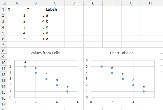
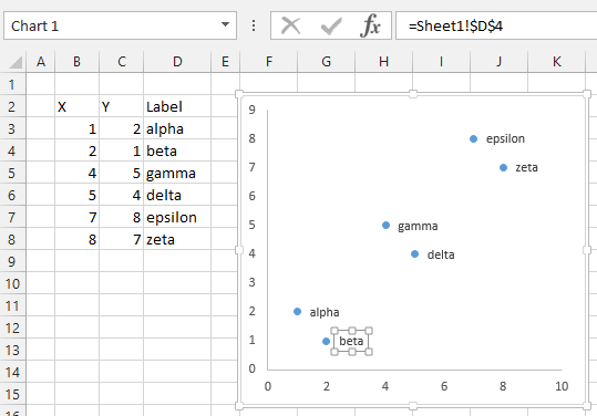
How to Add Labels to Scatterplot Points in Excel - Statology Step 3: Add Labels to Points. Next, click anywhere on the chart until a green plus (+) sign appears in the top right corner. Then click Data Labels, then click More Options…. In the Format Data Labels window that appears on the right of the screen, uncheck the box next to Y Value and check the box next to Value From Cells.

Change the format of data labels in a chart
Chapter 2 Simnet Flashcards | Quizlet display the data labels on this chart above the data markers you launched the chart elements menu, in the mini toolbar in the data labels menu, you clicked the above menu item display the data table, including the legend keys you launched the chart elements menu. In the mini toolbar in the data take menu, you clicked the with legend keys menu item
/Capture-e92aa05671d543ceaf94080eb2687619.JPG)
Understanding Excel Chart Data Series, Data Points, and Data ...
True an excel formula always begins with an equal - Course Hero See Page 1. TRUE An excel formula always begins with a (n)EQUAL SIGN =. Keyboard ___ can help youwork faster and more efficiently because you can keep your hands on the keyboard. payment required in each period to pay back the loan. SHORTCUTS The advantage of an electronic ___ is that the content can beeasily edited and updated to reflect ...

Pharmacological blood pressure lowering for primary and ...
quizlet.com › 515590718 › data-analytics-chapter-3Data Analytics Chapter 3: Describing data visually ... - Quizlet 4. to avoid graph clutter, numerical labels usually are omitted on a line chart, especially when the data cover many time periods. Use gridlines to help the reader read data values 5. data markers (squares, triangles, circles) are helpful. but when the series has many data values or when many variables are being displayed they clutter the graph

CIS Ch3 Excel Flashcards | Quizlet
Legends in Chart | How To Add and Remove Legends In Excel Chart? - EDUCBA Click on the chart so that it will be highlighted as below. Click on the "+" symbol on the top right-hand side of the chart. It will give a popup menu with multiple options as below. By default, Legend will be select with a tick mark. If we want to remove the Legend, remove the tick mark for Legend.
Adding data labels to see the value of the bars in an Excel chart
How to Choose the Right Chart for Your Data - Infogram Dual Column Chart- This dual axis column chart shows two sets of data displayed side by side. Multiple Axes Chart - This displays the most complex version of the dual axis chart. Here you see three sets of data - with three y-axes. Area Chart. Area charts are a lot like line charts, with a few subtle differences.

CIS Ch3 Excel Flashcards | Quizlet
Present your data in a doughnut chart - support.microsoft.com To make the data labels stand out better, do the following: Click a data label once to select the data labels for an entire data series, or select them from a list of chart elements ( Format tab, Current Selection group, Chart Elements box). On the Format tab, in the Shape Styles group, click More , and then click a shape style.
Apply Custom Data Labels to Charted Points - Peltier Tech
How to use data labels in a chart - YouTube Excel charts have a flexible system to display values called "data labels". Data labels are a classic example a "simple" Excel feature with a huge range of o...
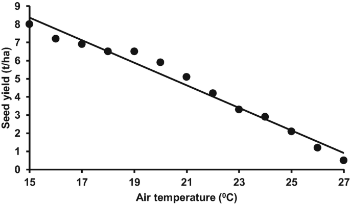
Effect of Low Temperature on Dry Matter, Partitioning, and ...
quizlet.com › 327118939 › ch-3-assessment-excel-2016Ch. 3 Assessment Excel 2016 IP Flashcards | Quizlet Study with Quizlet and memorize flashcards containing terms like Change the shape outline color to Orange, Accent 2. It is the sixth option in the first row of the color palette., Insert a Line chart based on the first recommended chart type., Insert a Waterfall chart based on cells A1:B10. and more.

Nanoparticulate Drug Delivery to the Retina | Molecular ...
Unit 11: Communicating with Data, Charts, and Graphs 11 Introduction. In every aspect of our lives, data—information, numbers, words, or images—are collected, recorded, analyzed, interpreted, and used. We encounter this information in the form of statistics too—everything from graphs of the latest home sales figures to census results, the current rate of inflation, or the unemployment rate.
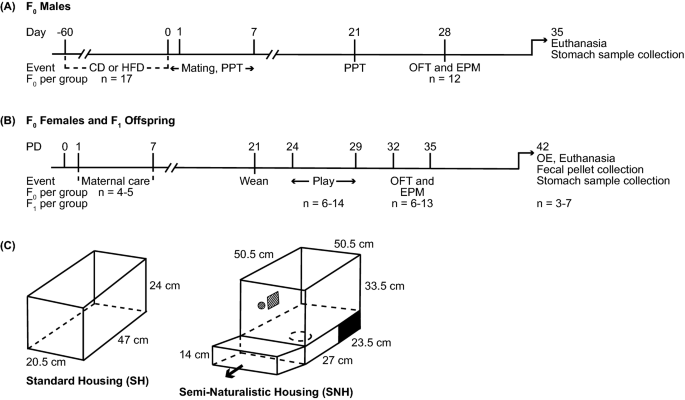
Effects of paternal high-fat diet and maternal rearing ...
Present data in a chart - support.microsoft.com Charts are used to display series of numeric data in a graphical format to make it easier to understand large quantities of data and the relationship between different series of data. 1. Worksheet data. 2. Chart created from worksheet data. Excel supports many types of charts to help you display data in ways that are meaningful to your audience.
Excel Chapter 4 review Flashcards | Quizlet
Solved 2 6 You want to create a pie chart to show the - Chegg 100% (13 ratings) Steps 2 - 6: Select A5:A10 and F5:F10 and Click Insert Menu --> Click Pie --> Select 2-D Pie - Move the chart to seperate sheet as named in the question Select the Chart --> Click Layout --> Click Chart Title --> CLick Above Chart - Enter the given T … View the full answer
microsoft excel - How do I reposition data labels with a ...
quizlet.com › 343637424 › misc-211-final-flash-cardsMISC 211 Final Flashcards | Quizlet Study with Quizlet and memorize flashcards containing terms like Use AutoSum to enter a formula in the selected cell to calculate the sum., Cut cell B7 and paste it to cell E12, Enter a formula in the selected cell using the SUM function to calculate the total of cells B2 through B6 and more.

CIS Ch3 Excel Flashcards | Quizlet
How to make a histogram in Excel 2019, 2016, 2013 and 2010 - Ablebits.com So, let's get to it and plot a histogram for the Delivery data (column B): 1. Create a pivot table To create a pivot table, go to the Insert tab > Tables group, and click PivotTable. And then, move the Delivery field to the ROWS area, and the other field ( Order no. in this example) to the VALUES area, as shown in the below screenshot.
Apply Custom Data Labels to Charted Points - Peltier Tech
Overview of PivotTables and PivotCharts - support.microsoft.com PivotCharts display data series, categories, data markers, and axes just as standard charts do. You can also change the chart type and other options such as the titles, the legend placement, the data labels, the chart location, and so on. Here's a PivotChart based on the PivotTable example above. For more information, see Create a PivotChart.
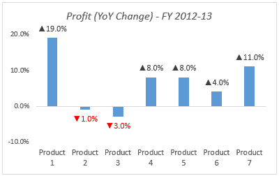
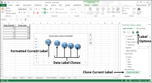
Color Negative Chart Data Labels in Red with downward arrow
CIS Ch3 Excel Flashcards | Quizlet Apply the Monochromatic Palette 2 color scheme from the Monochromatic section.. Add data labels to the selected pie chart. Add a trendline to the chart. Switch the data series with the categories on this chart. 1. change the selected chart to cluster column chart. 2. change the selected chart to cluster column chart.

CIS Ch3 Excel Flashcards | Quizlet
How to Place Labels Directly Through Your Line Graph in ...
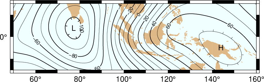
18. Annotation of Contours and “Quoted Lines” — GMT 6.1.1 ...

Display Customized Data Labels on Charts & Graphs

CIS Ch3 Excel Flashcards | Quizlet

Data Labels in FlexChart | Features | Wijmo Docs

CIS Ch3 Excel Flashcards | Quizlet

CIS Ch3 Excel Flashcards | Quizlet

Add or remove data labels in a chart
Chapter 11 Data visualization principles | Introduction to ...

CIS Ch3 Excel Flashcards | Quizlet
Excel 2016: Charts

Interactive Chart Tool | Alteryx Help

CIS Ch3 Excel Flashcards | Quizlet
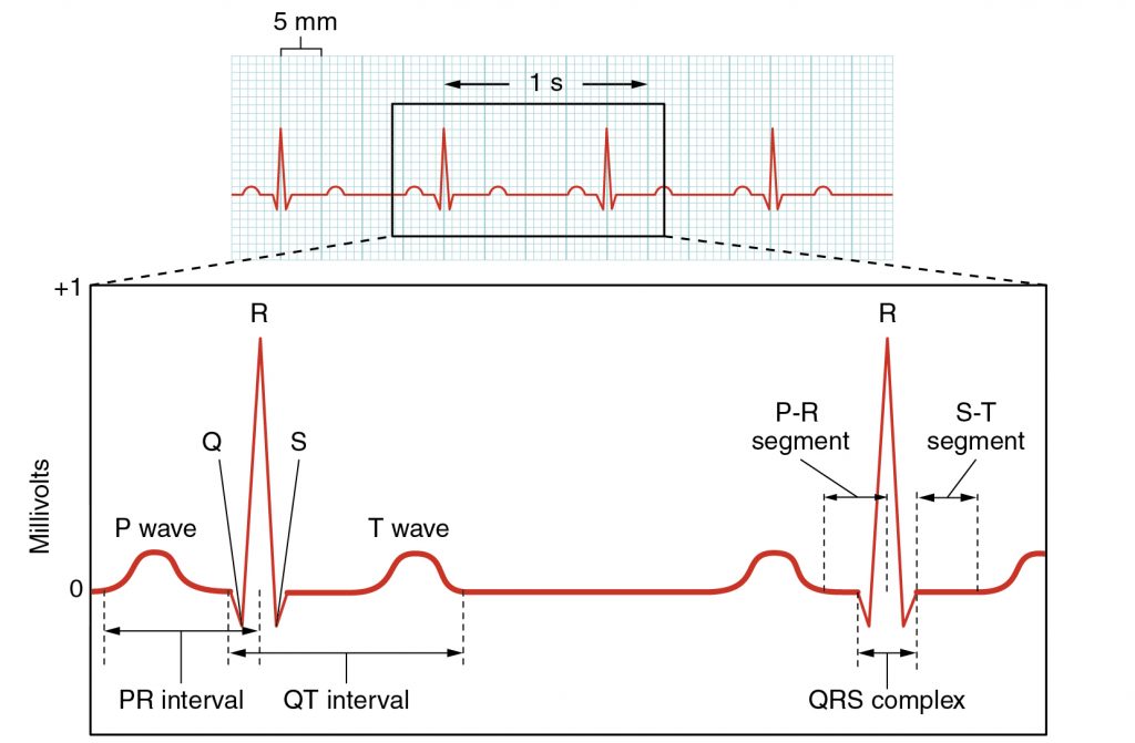
Assessment of Cardiovascular Function – A Mixed Course-Based ...

How to Place Labels Directly Through Your Line Graph in ...
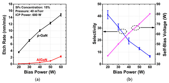
Micromachines | Editor's choice
Excel Charts - Aesthetic Data Labels

How to add data labels from different column in an Excel chart?
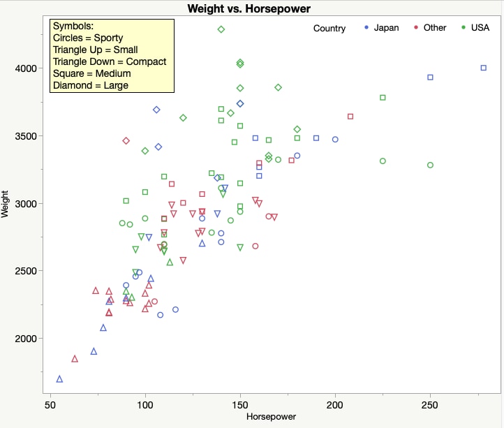
Scatter Plot | Introduction to Statistics | JMP

CIS Ch3 Excel Flashcards | Quizlet

Adding rich data labels to charts in Excel 2013 | Microsoft ...
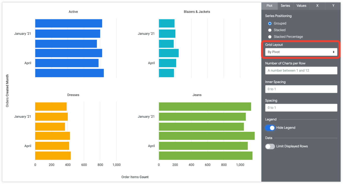
Bar chart options | Looker | Google Cloud
Post a Comment for "39 display the data labels on this chart above the data markers quizlet"